# Probability Theory We'll cover just enough of probability theory to get you ready for an interview, and hopefully not enough to bore you. I'll do my best to keep things concise but intuitive. But today will be a bit of an information dump. --- ## Random Variables We've said probability is to finance people what geometry is to architects. So how did people come up with geometry? Well first you decide on some concepts you care about. There's 3 dimensions so we measure how 'big' things are using length, width and height. All object will have these. Then we need a method to assign numbers to these values we care about. Well say we define some small increments - call them centimetres (or inches, depends where you're reading from), and measure everything else as multiples of those. How long something is = how many of these units you can fit in. That's what a ruler does. Probability is no different. Let's do the same thing with random events as we did with objects. We want some measure of how *likely* events are. So we define **Sample Space $\Omega$** as the set of all things that can happen. Then, **Random Variables** are statements about events that you can measure. So e.g. a *number of heads when tossing a coin 3 times* is a number you can measure. So is *temperature in New York tomorrow at 3PM*. This is the equivalent of length, width, or height as concepts. The set of all statements you can measure is called a *sigma algebra*. We denote it $\Sigma$. These variables can be *discrete* or *continuous*. Discrete have finite number of outcomes - e.g. the number of heads you saw when you flipped 3 coins. Continuous have infinitely many possibilities - e.g. *temperature in New York tomorrow at 3PM*. It can be 21°C, or 21.1°C, or 21.00001°C... infinitely many decimals. It's like the difference between integers and real numbers. ## Probability Then, we need a way to measure likelihood. Just like we had a ruler for length, width and height. We define **probability** - a map from the set of all measurable events (sigma algebra) to a number in [0, 1]. So any event you can measure will get a number between 0 and 1, that measures how likely the event is. The bigger the number, the more likely the event. Probability 0 means it's definitely not happening, probability 1 means it's sure to happen. The sum of probabilities of all events is 1, because *something* is sure to happen: $$\sum_{x\in \Sigma}P(x) = 1$$ We tend to think of probability as the frequency of how often something occurs. So in practice we define probability of an outcome as the number of ways it can occur, divided by the number of possible outcomes: $$P(\text{outcome})=\frac{\text{number of ways outcome can occur}}{\text{number of possible outcomes}}$$ So if you're tossing a coin, probability of getting heads is $\frac{1}{2}$. There's 1 successful out of 2 possible outcomes. Issue is, this definition doesn't nicely extend to continuous variables. Because you can have infinitely many outcomes, so denominator goes to infinity. Probability of any one outcome is 0. Instead, we define the probability of a continuous variable being in a certain range as: $$P(X\in[A,B])=\int_A^B f_X(x) dx$$ This $f_x(x)$ is called the **probability density** function (PDF). You can think of it like the probability measure for continuous random variables. And just like probability function summed up to 1 over all possibilities, PDF integrates to 1: $$\int_{-\infty}^{+\infty} f_X(x) dx=1$$ ## Set Properties You can think of events as different sets, and their probabilities as the surface. That way, we can make use of set properties.  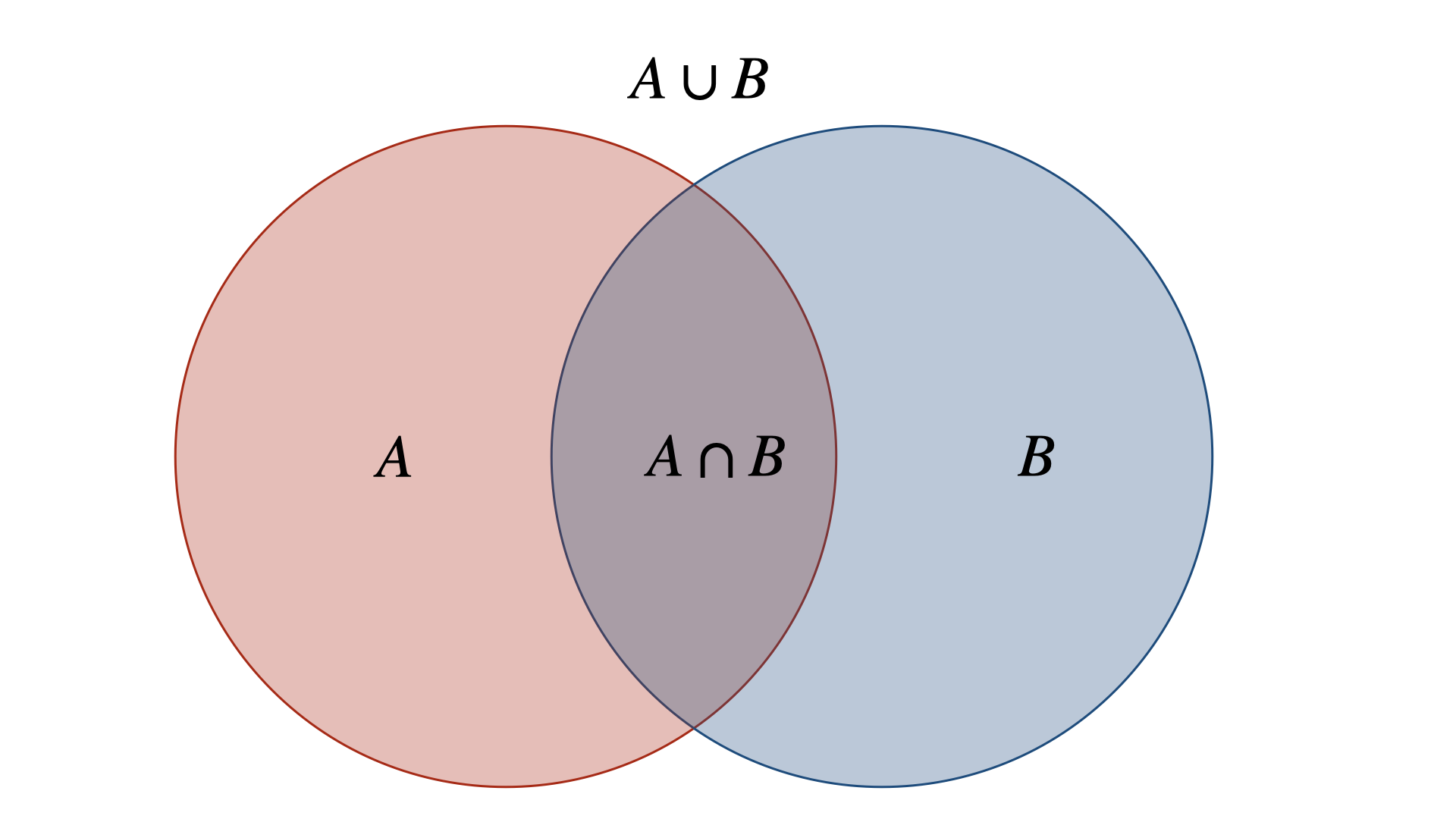$$P(A\cup B)=P(A) + P(B) - P(A\cap B)$$ Or, when events can't happen at the same time, $P(A\cap B)=0$ and $P(A\cup B)=P(A)+P(B)$. **Complement** of event A is simply everything that happens when event A doesn't. Their probabilities sum up to 1. We use this often in brainteasers, when probability of one or the other is easier to compute. $$P(A)+P(A^c)=1$$ We can find the probability of two events co-occuring as: $$P(A\cap B)=P(B|A)P(A) = P(A|B) P(B)$$ Where P(A|B) means probability of A given that event B happens. We can put these together into a **law of total probability**. It says: to find the chance of an event, split the world into all possible scenarios, find the chance in each scenario, then add them up: $$P(A) = \sum_i P(A|B_i)P(B_i)$$ Intuitively: it’s like asking “What’s the total chance it rains?” by adding up “chance it rains if it’s summer × chance of summer” + “chance it rains if it’s winter × chance of winter". <div style="display: flex; justify-content: space-between; align-items: baseline;"> <h2>Interview Question</h2> <span style="font-size: var(--font-s); font-style: italic; color: #333;">Jane Street</span> </div> --- If there's a 20% chance of it raining on Saturday and 30% chance of Sunday, what's the probability it rains this weekend? <div> <button class="toggle-solution">Show Solution <i class="fa-solid fa-chevron-down"></i></button> <div class="solution"> Let's use the set properties we've just derived. For it to rain during the weekend, it can either only rain on Saturday, only rain on Sunday or it can rain on both Saturday or Sunday. We know the chance of raining on Saturday is 20% (note this is not the same as 'Saturday only') and on Sunday it is 30%. If we were to add these, we'd double-count the chance of raining on both Saturday and Sunday once. To convince yourself why, simply draw the Venn diagrams of the different outcomes: <br><br><img src="/static/images/q105img1.png" alt="q105img1"><br><br>As we saw, you can think of probabilities of these events as surfaces of the different sections of the diagram. Denoting the chance of rain on Saturday A and Sunday B, we can find the probability of rain over the weekend as:<br><br>$$P(A\cup B) = P(A) + P(B) - P(A\cap B)$$<br><br>Now we already know $P(A)=0.2$ and $P(B)=0.3$, so how can we find $P(A\cap B)$? We can safely assume that rain on Saturday and rain on Sunday are independent events, such that $P(A\cap B)=P(A)\cdot P(B)=0.06$. Therefore, $P(A\cup B)=0.2 + 0.3 - 0.06=0.44$. </div> </div> ## Conditional **Conditional probability** is about updating your view once you know something happened. Instead of asking, “What’s the chance of rain today?” you ask, “What’s the chance of rain given I see dark clouds?”. The formula comes from the expression we saw for $P(A\cap B)$: $$P(A|B)=\frac{P(B|A)P(A)}{P(B)}$$ This topic comes up on interviews a lot, so it pays to remember the formula. ## Cumulative Distribution Function CDF is the chance your variable takes value at most x. For discrete variables: $$P(X\leq x)=\sum_{X\leq x}P(X=x)$$ Or in the case of continuous variables: $$P(X\leq x) =\int_{-\infty}^xf_X(x) dx$$ When you're asked to derive PDF of some variable, it's often easier to first derive CDF and take a derivative. For example, to find the distribution of max of a number of variables. If max of a group is smaller than some x, then each element in the group is below x. So $P(max(X_i)\leq x)=P(X_1\leq x)\cdot P(X_2\leq x)...P(X_n\leq x)=P(X_i\leq x)^n$. That way, if you know CDF of one of the variables, you can easily find CDF of the max. Similar story for the minimum, except if $min(X_i)\geq x$ then $X_i\geq x$ for all i. You then simply express $P(min(X_i)\geq x)=1-P(min(X_i)\geq x)$ in terms of the CDF. ## Expected Value Now if you had to guess what the future outcome of a random variable will be, what should you guess? Well you could take all the outcomes, weight them by how likely you are and sum. That's what expected value is. For discrete variables: $$E(X)=\sum_i X_i \cdot P(X_i)$$ And similarly in the continuous case the sum just turns to an integral: $$E(X)=\int_{-\infty}^{+\infty} x f_X(x) dx$$ Note that expectation is *linear*, so: $$E(aX+bY) = aE(X) + bE(Y)$$ And when two variables are *independent* (we'll explain this shortly): $$E(XY)=E(X)\cdot E(Y)$$ Lastly, note that expectation naturally extends to functions of random variables: $$E(g(X))=\sum_i P(X_i) g(X_i)$$ ## Variance Now once you've made a guess, say you're asked how sure you are about your guess. You could look at each possible outcome, and see how far away it is from your best guess on average. Except that you care about absolute distance (smaller or bigger), so you don't want negative distances to reduce your variance. The more dispersed / messy the points, the higher you want this number. So we'll square the distance instead, to look at pure length. This is what variance is. For the discrete case: $$Var(X)=E((X-E(X))^2) = \sum_i P(X_i) (X_i-E(X))^2$$ Or in the continuous case: $$Var(X)=\int_{-\infty}^{+\infty} (X-E(X))^2 f_X(x)$$ Another way to write this, which is more commonly used in problems is: $$Var(X)=E(X^2)-E(X)^2$$ Variance is a quadratic operator: $$Var(aX + b)=a^2 Var(X)$$ Here a and b are constants. Note also we call the square root of variance **standard deviation**: $$\sigma(x) = \sqrt{Var(X)}$$ ## Covariance & Correlation Sometimes you'll see random variables that tend to move in tandem. It's like they follow each other. So e.g. if you were to track ice cream sales and temperature, you'd find that high temperature seems to lead to high ice cream sales, and vice-versa. This is called *correlation*. We define it as: $$Cov(X,Y)=E(XY)-E(X)E(Y)$$ Notice that if you just plugged in two X into this formula, you'd recover variance: $$Cov(X,X)=Var(X)$$ This is quite useful to solve for variance of complicated expressions. Because you can split up covariance nicely: $$Var(aX+bY)=cov(aX + bY, aX+bY)=cov(aX, aX)+2 cov(aX,bY) + cov(bY, bY)=$$ $$=a^2 Var(X) + 2ab\cdot cov(X,Y)+ b^2 Var(Y)$$ So covariance tells you how much two variables vary together. It tells you the direction (can be positive or negative), and it depends on individual variances of the two variables. So if one variable has huge variance (big ups and downs), the covariance number can look large even if the relationship isn’t that tight. That's why we use often use **correlation**: it divides by the standard deviations of each variable, removing the “inflation” from individual variability and leaving only the true strength of co-movement: $$cor(X,Y)=\frac{cov(X,Y)}{\sqrt{Var(X)Var(Y)}}$$ Correlation always falls between -1 and 1. ## Executive Summary - **Random Variables:** like measuring length with a ruler, random variables measure outcomes. Discrete ones take countable values (coin flips), continuous ones take infinitely many (temperature). - **Probability:** assigns each measurable event a number between 0 and 1. Discrete case = number of favorable outcomes divided by total. Continuous case = area under a probability density function. Probabilities of all outcomes sum (or integrate) to 1. - **Set Properties:** probabilities behave like areas of sets. Union = add probabilities but subtract overlap. Complement = everything outside an event. Conditional probability updates likelihood once you know another event happened. - **Law of Total Probability:** split the world into scenarios, compute chance in each, and add them up. Like asking “what’s total chance it rains?” by adding summer × chance of summer + winter × chance of winter. - **Expected Value:** weighted average of possible outcomes, using probabilities as weights. It’s linear, and for independent variables, $E(XY)=E(X)E(Y)$. - **Variance & Standard Deviation:** measure how spread out outcomes are from the mean. Variance = expected squared distance from mean. Standard deviation = square root, giving spread in original units. - **Covariance & Correlation:** covariance measures how two variables move together, but can be inflated by scale. Correlation normalizes this, giving a pure measure of co-movement between -1 and 1.