# Distributions Distributions of random variables tell you how likely each possible value is — it shows which outcomes happen often, which are rare, and how the chances are spread out. There are different distribution families. We'll see examples of a few most important. --- ### Discrete Uniform Distribution If you roll a 6-sided die once, there's 6 possible outcomes - and all are equally likely. This is a **(discrete) uniform** distribution. It's characterised by a finite number of outcomes, all of which are equally probable. So if you have $N$ possible outcomes, probability of any one is: $$P(X)=\frac{1}{N}$$ Let's find the expected value: $$E(X) = \frac{1}{N}\sum_{i=1}^N i = \frac{1}{N}\frac{N (N+1)}{2}=\frac{N+1}{2}$$ Here we used the well-known formula for the sum of first N numbers: $\frac{N (N+1)}{2}$. There's also a formula for the sum of first N numbers squared: $\sum_{i=1}^N i^2 = \frac{N(N+1)(2N+1)}{6}$. We'll need this to find the variance: $$Var(X) = E(X^2)-E(X)^2 = \frac{1}{N}\sum_{i=1}^N i^2 - E(X)^2=$$ $$=\frac{(N+1)(2N+1)}{6} - \frac{(N+1)^2}{4}=\frac{(N+1)(N-1)}{12}$$ ### Continuous Uniform Distribution There's also a similar concept for continuous random variables. Here random variables can take values within some interval [a,b]. And probability density function is constant along the entire interval. Namely: $$f_X(x)=\frac{1}{b-a}$$ Then expected value is: $$E(X) = \int_a^b x \frac{1}{b-a}dx =$$ $$=\frac{1}{b-a} \frac{b^2-a^2}{2}=\frac{b+a}{2}$$ And the variance is: $$Var(X)=\int_a^b \left(x-\frac{a+b}{2}\right)^2 \frac{1}{b-a}dx$$ $$=\frac{(b-a)^2}{12}$$ ## Binomial Distribution Now imagine you're tossing a fair coin $n$ times. The probability of tossing $X$ heads (or tails) belongs to the **binomial distribution**. Generally, if you have $n$ trials, each with two possible outcomes—one occurring with probability $p$ and the other with probability $1-p$ — then the probability of observing $X$ successful outcomes is: $$P(X=x)=\binom{n}{x}p^x (1-p)^{n-x}$$ The expected value for binomial distribution is: $$E(X)=np$$ While its variance is: $$Var(X)=np(1-p)$$ <div style="display: flex; justify-content: space-between; align-items: baseline;"> <h2>Interview Question</h2> <span style="font-size: var(--font-s); font-style: italic; color: #333;">Goldman Sachs</span> </div> --- Can you compute the expected value and variance of a binomial $Bin(n,p)$ distribution? Recall that it is a sum of n independent Bernoulli trials, all of which take value 1 (win) with probability $p$ and 0 (loss) with probability $1-p$. <div> <button class="toggle-solution" >Show Solution <i class="fa-solid fa-chevron-down"></i></button> <div class="solution"> Let's assume you don't remember any distribution-specific formulas and derive these ground up. We are asked for expected value of a binomial distribution, which is itself a sum of independent variables. We know that expectation is additive, i.e. $E(X+Y) = E(X) + E(Y)$, and so is variance in the case of independent variables (since covariance term goes to 0), i.e. Var(X+Y) = Var(X) + Var(Y). Then, if we compute the expected value and variance of the Bernoulli trial, we can sum them up to get to Binomial.<br><br>Bernoulli trial $X$ can be 1 with probability $p$ and 0 with probability $1-p$ so its expected value is $E(X) = p\cdot 1 + (1-p)\cdot 0 = p$. Its variance is $Var(X) = E(X^2) - E(X)^2$. We already know the second term, since we know the expectation. As for the first term, notice that in the case of a Bernoulli trial, $X=X^2$, i.e. if $X=1$ then $X^2=1$; if $X=0$ then $X^2=0$. Then, we have $Var(X) = E(X) - E(X)^2 = p(1-p)$.<br><br>Now that we know the Bernoulli trial parameters, we simply sum up to binomial. Assuming $Y\sim Bin(n,p)$, then $Y = \sum_{i=1}^n X_i$ with $X_i$ Bernoulli trials. $$E(Y) = \sum_{i=1}^n E(X_i) = np$$ $$Var(Y) = \sum_{i=1}^n Var(X_i) = np(1-p)$$ </div> </div> ## Normal (Gaussian) Distribution This is probably the most important distribution to know. Finance people use it all the time, to model changes in price. It also occurs a lot in nature. Say you were to measure the height of a group of people. Their height is normally distributed. 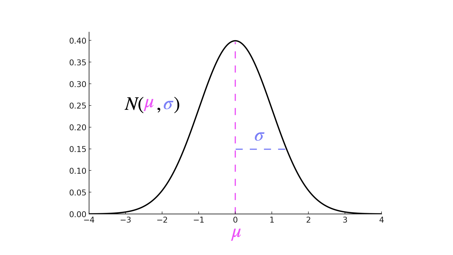The probability density function of this family has the famous bell shape:  The intuition is: most people have height close to the average $\mu$. Very few people are very short / tall, so probability drops off as you move into the extremes. How quickly it drops off is dictated by the $\sigma$ - standard deviation parameter. The bigger the $\sigma$, the further from the mean you can see values with high probability. We denote normal distribution with parameters $\mu$ and $\sigma$ as $N(\mu, \sigma)$. The expected value of a normal variable is: $$E(X)=\mu$$ And its variance is: $$Var(X)=\sigma^2$$ The probability density function (PDF) of a normal variable is: $$f_X(x) = \frac{1}{\sqrt{2\pi\sigma^2}}e^{-\frac{(x-\mu)^2}{2\sigma^2}}$$ # Statistics We've now seen the probability theory. But to use this to talk about real events, we need statistics. Just like architects use rulers to attribute concepts of length, width and height to objects before they can do geometry. You can think of it like this: probability said 'given X probability family, Y event has probability Z'. Then statistics says: 'given Z data, event Y seems to behave like X probability family'. So recall how we said people's heights tend to be normally distributed. It sounds right in theory - most people have average height, and then very few are very tall / very short. But how can we test this? That's what we'll try to get to in the following sections. --- ## Random Sample Firstly, you'd go and get a group of people to measure their height. We'd consider these people as random variables that actually realised. This set of realised random variables from the same family distribution is called a **random sample**. We often assume random sample is *i.i.d = independent and identically distributed* set of variables. 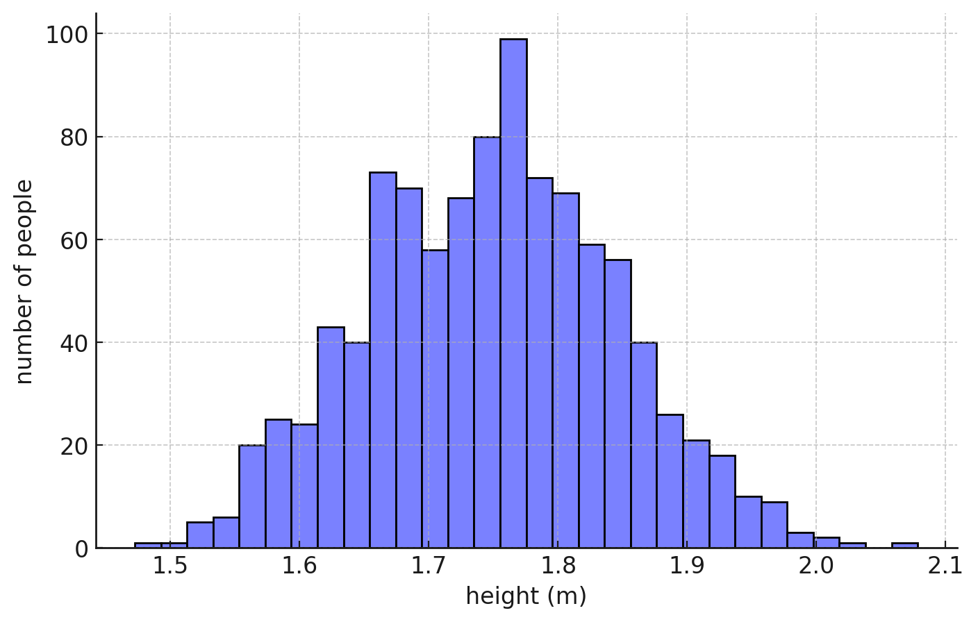Then we'd go and plot them, and say we see something like this:  Okay, so it looks like indeed most people have average height, and you have a few very tall and very short outliers. So you can probably conclude that, if you take another person, their height would follow a normal, bell-shaped distribution. And say we want to actually predict, what's the most likely height of a random person, or what's the chance he's 2m tall. If we knew the exact parameters $\mu$ and $\sigma$ in the $N(\mu, \sigma)$ distribution that people's height follows, we could do that. Looking at the plot, you can probably guesstimate that average is around 1.7-1.8. But can we make this precise? Yes! That's what **estimators** do. ## Estimators Estimators are functions of observations in a random sample that should approximate the parameters of the underlying distribution. That's to say, imagine there is really this hidden Normal distribution $N(\mu, \sigma)$ that spits out human heights - what would be its mean and variance? Note that these distributions are a theoretical concept we impose on real data, in order to make sense of it and produce good guesses. There isn't really an underlying processes drawing from a normal distribution every time a baby is born. The simplest estimator for mean $\mu$ if you have $n$ variables is: $$\overline{\mu}=\frac{1}{n}\sum_{i=1}^n X_i$$ Note that $X_i$ are in principle random variables, which we assume come from $N(\mu, \sigma)$ distribution. So $\overline{\mu}$ is also a random variable. Don't confuse the fact we're calling $X_i$ random variables with the fact we're measuring real human heights. We're constructing this estimator to work on random variables. Then, in order to use it - we will observe real data, which we view as realisations of random variables. Get it? Then, if $\overline{\mu}$ is a random variable that should give you a good estimate of $\mu$, we would expect its expected value to be $\mu$, right? On average, this estimator should give you a good approximation of $\mu$. Let's test this: $$E(\overline{\mu}) = \frac{1}{n}\sum_{i=1}^n E(X_i)$$ Now remember our assumption is that $X_i \sim N(\mu, \sigma)$, so $E(X_i)=\mu$. We get: $$E(\overline{\mu})=\frac{1}{n}n\cdot \mu=\mu$$ Okay, cool - so our estimator on average gives us $\mu$ - the value it's constructed to estimate. That's a good estimator - in practice called **unbiased estimator**. <div style="display: flex; justify-content: space-between; align-items: baseline;"> <h2>Interview Question</h2> <span style="font-size: var(--font-s); font-style: italic; color: #333;">Goldman Sachs</span> </div> --- Explain what is an unbiased estimator? <div> <button class="toggle-solution" >Show Solution <i class="fa-solid fa-chevron-down"></i></button> <div class="solution"> As we've seen, unbiased estimator $W$ of parameter $\theta$ is an estimator whose expected value equals the parameter itself, i.e. $E(W)=\theta$. </div> </div> Estimators also have variance. It shows us how uncertain they are. The higher the variance, the less reliable your estimator. $$Var(\overline{\mu})=\frac{\sigma^2}{n}$$ So if you now observe real human heights, you can sum them up and divide with the number of observations, and that should be a pretty good guess of the mean height $\mu$. And since we assumed heights follow a normal distribution, this is also your best guess for the height of a random person you haven't yet seen. Now we can also estimate variance $\sigma^2$, to see how much people's heights tend to vary from the average. We have an estimator for this too: $$S^2=\frac{\sum_{i=1}^n(X_i-\overline{X})^2}{n-1}$$ Notice we're dividing by $n-1$ instead of by $n$. This is because one data point was already “spent” to calculate the mean, so only n-1 pieces of information remain to measure how spread out the data really is. This is also an unbiased estimator, so that: $$E(S^2)=\sigma^2$$ *Attention* Don't confuse estimator of the variance with variance of the estimator, or estimator of the expectation with expectation of the estimator. ## Central Limit Theorem In practice, we don't always know the exact distribution of statistical estimators. Especially if the functions are more complex and when the underlying data doesn't come from a 'nice' distribution like Gaussian. This is why **Central Limit Theorem** is handy. It tells you that sample mean $\overline{X}=\frac{1}{n}\sum_{i=1}^n X_i$ is always normally distributed given a big enough $n$ - whatever the underlying distribution! Formally, if you take $X_1, X_2, ..., X_n$ from any distribution with constant mean $\mu$ and finite variance $\sigma^2$, then normalised sample mean approaches *standard normal* distribution as $n\rightarrow \infty$: $$\frac{\sqrt{n}(\overline{X}-\mu)}{\sigma}\rightarrow N(0,1)$$ Most estimators will use sample mean $\overline{X}$, so this is quite a handy feature. But that's not why we care about it now - interviewers sometimes ask you to define it / understand what it means, so remember it. ## Law of Large Numbers Another law you should be familiar with. Law of large number says that as the number of observations grows, the sample mean $\overline{X}=\sum_{i=1}^n X_i$ approaches the real mean $\mu$. I.e. the average approaches the expected value. Think of it like this: if you only take a couple of samples, chance plays a big role — you might get lucky or unlucky. But as you collect more and more samples, the lucky streaks and unlucky streaks cancel each other out. The average then settles down closer and closer to the true value. For example, tossing a coin 4 times might not give you 2H and 2T. You might well get 4H and no T. The underlying distribution where both heads and tails are equally likely is not represented. But tossing a coin 5,000 times will give you almost exactly half heads, half tails. ## Confidence Intervals Okay, so our estimators are actually random variables themselves. They have a mean, a variance, and a probability distribution. That means a single point estimate (like $\overline{X}=1.75$) is just one possible outcome — if we took another sample, we’d likely get a slightly different value. So instead of reporting just one number, we can give a **range of plausible values** for the true parameter. This is called a **confidence interval**. For example, we might say: "we are 95% confident that the true mean height $\mu$ lies between 1.72m and 1.78m." Formally, the idea is this: if we repeated the sampling process many times and each time built such an interval, about 95% of those intervals would contain the true parameter. It's not that the parameter itself is moving — it’s fixed — it’s that our estimate jumps around with the data, and the interval is wide enough to catch the truth most of the time. Mathematically, for the mean of a Normal distribution with variance $\sigma^2$ known, the confidence interval is: $$\overline{X} \pm z_{\alpha/2} \cdot \frac{\sigma}{\sqrt{n}}$$ Here $z_{\alpha/2}$ is the cutoff from the standard normal distribution (about 1.96 for 95% confidence). If $\sigma^2$ is unknown, we replace it with the sample variance and use the $t$-distribution instead: $$\overline{X} \pm t_{n-1,\alpha/2} \cdot \frac{S}{\sqrt{n}}$$ This way, we don’t just say “the average height is 1.75,” but rather “the average height is about 1.75, give or take 0.03,” which is a much more honest reflection of the uncertainty in our estimate. Make sure to understand this - for some reason, confidence intervals tend to appear often in interviews. <div style="display: flex; justify-content: space-between; align-items: baseline;"> <h2>Interview Question</h2> <span style="font-size: var(--font-s); font-style: italic; color: #333;">Goldman Sachs</span> </div> --- What is a confidence interval and how does it scale with the number of observations? <div> <button class="toggle-solution" >Show Solution <i class="fa-solid fa-chevron-down"></i></button> <div class="solution"> A confidence interval is a range of values, derived from sample data, that is likely to contain the true population parameter with a specified probability (the confidence level, typically 95% or 99%). The width of the confidence interval decreases as the number of observations increases because the standard error (which determines the margin of error) is inversely proportional to the square root of the sample size (n). Mathematically, the standard error scales as $\frac{1}{\sqrt{n}}$, meaning that quadrupling the sample size halves the standard error and, consequently, the width of the confidence interval. </div> </div> ## Executive Summary - **Uniform distribution:** all outcomes are equally likely. Discrete uniform (like rolling a fair die) has finite outcomes, continuous uniform (like picking a random number between a and b) has infinitely many. Mean is the midpoint, variance shrinks as the range gets tighter. - **Binomial distribution:** models number of successes in $n$ independent trials with success probability $p$. Probability of $x$ successes uses the formula with binomial coefficients. Expectation is $np$, variance is $np(1-p)$. - **Normal distribution:** the famous bell curve, used constantly in finance and nature. Most observations cluster around the mean $\mu$, with spread controlled by standard deviation $\sigma$. Expected value = $\mu$, variance = $\sigma^2$. - **Random sample:** a collection of independent draws from the same distribution (i.i.d). In practice, it’s how we gather data to estimate unknown parameters. - **Estimators:** formulas based on samples that approximate parameters of the true distribution. An estimator is **unbiased** if its expected value equals the true parameter. Sample mean estimates $\mu$, sample variance estimates $\sigma^2$. - **Central Limit Theorem:** sample means are approximately normal for large $n$, regardless of the original distribution. This is why normal distribution shows up everywhere in statistics. - **Law of Large Numbers:** as sample size grows, the sample mean approaches the true mean. Randomness cancels out when enough trials are taken. - **Confidence Intervals:** instead of one number, give a range where the true parameter likely lies (e.g. 95% of such ranges would contain the true value). The width shrinks with more data, at the rate $1/\sqrt{n}$.