# Brownian Motion
This is how we introduce randomness into classical maths. I'll only teach you the stuff you need for the interview. First a few names and properties you need to know - learn these by heart. Then some intuition on the weirdness - so you can show understanding without delving into proofs. And lastly a few tricks to answer real interview questions - you only need to see the tricks once and you'll remember them.
---
## Stochastic Process
Okay, so our task is to model the price. Take a look at any price chart - it's a mess. Modelling this with a smooth function would be a hard sell.
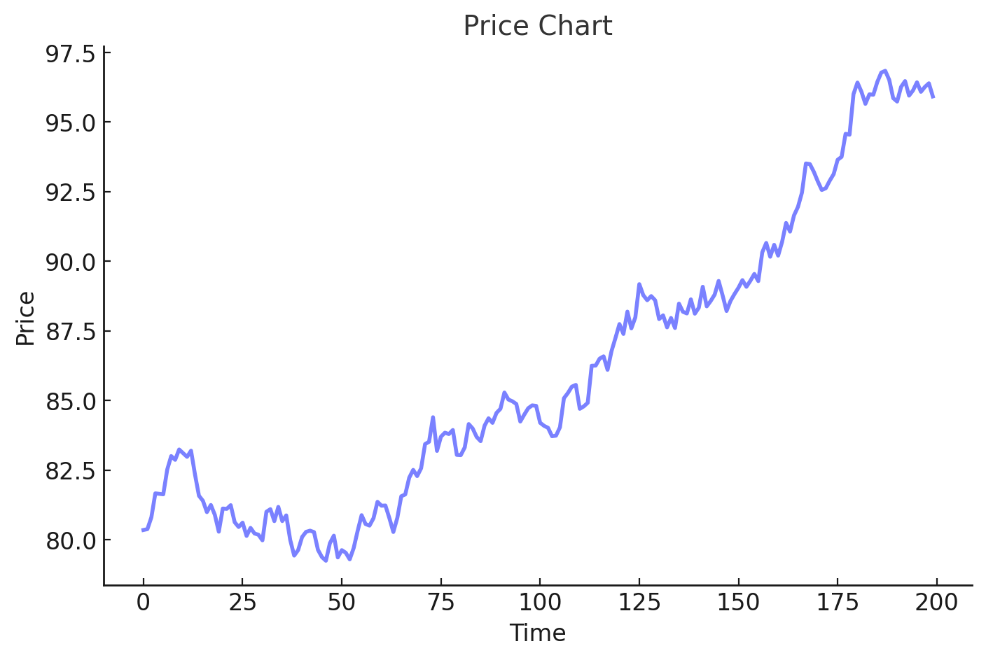
So how can we produce a messy, jumpy, random-looking pattern? Well random variables are random, so we could put together a bunch of them to form a time graph. In fact, this is what a **stochastic process** is - a collection of random variables indexed by time. We denote it as:
$$\\{ X_t \\}_{t \\geq 0}$$
## Filtration
This indexing by time is important: a random variable in the past has already realised - it's known. A random variable in the future is unknown. So we call the level of information you have at time $t$ a **filtration** $F_t$. A stochastic process $X_t$ is **adapted** to $F_t$ means you know variable $X_s$ at time $s$. It's a bit like how a movie is adapted to its timeline: at minute 0 you know nothing, at minute 1 you see the first scene and by minute 120 you've seen them all.
## Brownian Motion Definition
Brownian motion is a special kind of stochastic process: You start at 0, and then jump every time interval by a random amount. These random jumps are drawn from a Normal distribution centered at 0 with variance equal the time interval. 'Centered at 0' means you're most likely to jump a tiny amount, and less likely to jump a huge amount. 'Time interval variance' means the longer the time between jumps, the more likely the bigger jump is. One last thing - each jump is independent of the jumps before it. That's it.
<img src="/static/images/building_brownian_motion.png" alt="Probability Tree" style="max-width: 100%;">
Another name for this is Wiener's process - same thing.
If you denote brownian motion as $B$, and take two times $s$ and $t$ with $s>t$, we can formalise this as:
$B_0 = 0$ - you're starting at 0
$B_s-B_t \sim N(0,s-t)$ - jumps are drawn from a normal distribution
$B_s - B_t \perp F_t$ - jumps are independent of what came before
## Weird Properties
They might ask you about the following to check your understanding of how the process works:
*Brownian motion oscillates between positive and negative in any time interval you chose*. It's why visualisations like the graphs above are (sort of) misleading. Because we only picked certain points in time and evaluated brownian motion at those points. But for any tiny interval you pick, zoom in enough and you will see it oscillate between negative and positive values.<br><br>
What this means is ***you can zoom in as much as you like, and the chart won't get any smoother***.
<img src="/static/images/brownian_motion_differentiability.png" alt="Brownian Differentiability" style="max-width: 100%;">
The implication is **brownian motion is not differentiable**. Differentiable just means if you zoom in enough, the function starts to look like a straight line (like the smooth function in top row). Brownian motion stays chaotic at every level, so it's not differentiable.<br><br>Last thing to know is, *given enough time - brownian motion reaches both $+\infty$ and $-\infty$*. Therefore, it also *reaches any value $c$ in finite time*.
<div style="display: flex; justify-content: space-between; align-items: baseline;">
<h2>Interview Question</h2>
<span style="font-size: var(--font-s); font-style: italic; color: #333;">Goldman Sachs</span>
</div>
---
If $B_t$ is a brownian motion, find the $cov(B_t, B_s)$ and $cor(B_s, B_t)$ for $s>t$.
<div>
<button class="toggle-solution">Show Solution <i class="fa-solid fa-chevron-down"></i></button>
<div class="solution">
Recall the definitions: $$cov(B_s, B_t)=E(B_s\cdot B_t)-E(B_s)\cdot E(B_t)$$ $$cor(B_s, B_t)=\frac{Cov(B_s, B_t)}{\sqrt{Var(B_s)\cdot Var(B_t)}}$$So we first need to find the covariance. Note that $B_t$ can be written as $B_t-B_0$ because $B_0=0$ - the first property of brownian motion. Second property tells us that increment $B_t-B_0 \sim N(0,t)$, so its expected value $E(B_t)=E(B_t-B_0)=0$. Therefore $E(B_s)=E(B_t)=0$ and only the first term remains:
$$cov(B_s,B_t)=E(B_s\cdot B_t)$$
Notice we only have useful things to say about the increment $B_s-B_t$, so the goal is to express covariance in terms of this increment, so we can use its properties. We can simply add and subtract $B_t$ from $B_s$:
$$E(B_s\cdot B_t)=E((B_s-B_t+B_t)\cdot B_t)=E((B_s-B_t)\cdot B_t + B_t^2)$$
Now we know that $E(X+Y)=E(X)+E(Y)$ so we can decompose:
$$cov(B_s,B_t)=E((B_s-B_t)\cdot B_t)+E(B_t^2)$$
We also know that $E(XY)=E(X)E(Y)$ when $X$ and $Y$ are independent. Third property of brownian motion tells us that the increment $B_s-B_t$ is independent of all that happened up to time t ($F_t$), which includes $B_t$. So $B_s-B_t \perp B_t$ and therefore:
$$E((B_s-B_t)\cdot B_t)= E(B_s-B_t)\cdot E(B_t)$$
We already found that $E(B_t)=0$ so this term is 0. What remains is $cov(B_s,B_t)=E(B_t^2)$. Recall the definition of variance: $Var(B_t)=E(B_t^2)-E(B_t)^2$. But because for brownian motion $E(B_t)=0$, we have $Var(B_t)=E(B_t^2)$. We saw that we can write $B_t$ as the increment $B_t-B_0 \sim N(0, t)$ so that $Var(B_t)=t$. Then:
$$cov(B_s, B_t)=t$$
If we had started with assumption that $ s\lt $ instead of $s>t$ we would get $cov(B_s,B_t)=s$. So the general solution is $cov(B_s,B_t)=min(s,t)$.<br><br>To find covariance, we simply divide with square root of the two variances:
$$cor(B_s,B_t)=\frac{min(s,t)}{\sqrt{t\cdot s}}$$
</div>
</div>
## Alternative Definition
This is an important result, because you can use this property to define brownian motion. In fact, an alternative definition is:
**"Brownian motion is a continuous, centered (mean 0) Gaussian process $B_t$ such that $cov(B_s, B_t)=min(s,t)$"**
This is good to know because when they ask you to prove that some process is brownian motion, it's usually easier to show this property than the original three. Recall Gaussian = Normally Distributed.
<div style="display: flex; justify-content: space-between; align-items: baseline;">
<h2>Interview Question</h2>
</div>
---
If $B_t$ is a brownian motion, prove $t\cdot B_{1/t}$ is also a brownian motion.
<div>
<button class="toggle-solution" >Show Solution <i class="fa-solid fa-chevron-down"></i></button>
<div class="solution">
How can we prove something is a brownian motion? Well we either show the original three properties of brownian motion hold, or we can use the alternative definition. The alternative definition tends to be easier to prove, so let's try that.<br><br>
<b>1. Continuity</b> - we know $B_t$ is a brownian motion, so it is continuous for any $t$. Now $B_{1/t}$ is just this process evaluated at time $\frac{1}{t}$, so it's continuous. And $t$ is a constant so multiplying by it doesn't affect continuity. Therefore $X_t=tB_{1/t}$ is continuous.<br><br>
<b>2. Centered Gaussian</b> - we know $B_t$ is a centered Gaussian process, i.e. normally distributed with mean 0. As before, going from $t$ to $1/t$ changes nothing, as it's just the same process at a different time. And since $t$ is just a constant, then $E(X_t)=E(tB_{1/t})=tE(B_{1/t})=0$. Therefore, $X_t$ is a centered Gaussian.<br><br>
<b>3. Covariance</b> - we need to prove that $cov(X_t, X_s)=min(s,t)$, knowing this holds for $B_t$. We can develop the expression:
$$cov(X_t, X_s)=cov(tB_{1/t}, sB_{1/s})=t\cdot s \cdot cov(B_{1/t}, B_{1/s})$$
Now we know that for any times $\tilde{s}$ and $\tilde{t}$, $cov(B_{\tilde{t}}, B_{\tilde{s}})=min(\tilde{t}, \tilde{s})$. So setting $\tilde{t}=\frac{1}{t}$ and $\tilde{s}=\frac{1}{s}$, we know $cov(B_{1/t},B_{1/s})=min(1/t, 1/s)$. Therefore we conclude:
$$cov(X_t, X_s)=t\cdot s \cdot min(1/t, 1/s)=min(t\cdot s/t, t\cdot s /s)=min(t,s)$$
This was the last of the three properties. We conclude $X_t$ is a brownian motion.<br><br>
To make sure you've got this, try the same problem with $X_t=\frac{1}{c}B_{c^2 t}$ with $c$ a constant.
</div>
</div>
## Executive Summary
<div class="executive-summary">
<h3>New Definitions</h3>
<b>Stochastic Process</b> - a collection of random variables indexed by time.<br><br>
<b>Filtration</b> - level of info you have at any time.<br><br>
<b>Adapted Process</b> - collection of random variables that's revealed incrementally as time goes on.<br><br>
<b>Brownian Motion</b> - adapted process that starts at 0, moves in normally-distributed increments which are independent from the past.
<h3>Behaviour & Intuition</h3>
Brownian motion looks messy however much you zoom in.<br><br>
It is <b>not differentiable</b>.<br><br>
It reaches any level (including $+\infty$ and $-\infty$) in finite time.<br><br>
It oscillates between positive and negative in any interval you chose.
<h3>Problem Solving Tricks</h3>
To derive properties of $B_t$, write $B_t=B_t-B_0$ and use what you know about the increment (Gaussian, independent of $F_t$).<br><br>
To show something's a brownian motion, either show the three main properties, or show it's continuous, centered Gaussian process with $cov(X_t, X_s)=min(t,s)$.<br><br>
To work with expressions like $B_t\cdot B_s$, add and substract to form increments: $$B_s\cdot B_t=(B_s-B_t)\cdot B_t+B_t^2$$
That way you have independent Gaussian terms, as increment is Gaussian and independent of what came before it.
</div>